This is a key component of the PLONK protocol. Before diving in, let's explore the term "arithmetization" in the context of zero knowledge.
Arithmetization is the process of converting computational statements into mathematical equations, specifically polynomial equations, that can be efficiently proven and verified. It's like translating a computer program into a mathematical language that zero-knowledge proofs can understand.
These are the basic building blocks of arithmetization:
- Variables: represent values in the computation
- Constraints: mathematical relationships between variables
- Polynomials: used to encode relationships and checks
- Fields: mathematical structures where the computation occurs
Over the years, many forms of arithmetization have been laid out. Let's explore a few.
Rank-1 Constraint System (R1CS)
- Used in protocols like Groth16
- Represents a computation as $Ax \circ Bx = Cx$, where $A, B, C$ are matrices, $x$ is the witness vector, and $\circ$ is element-wise multiplication
Plonkish arithmetization
- Used in PLONK and its variants
- Gate format: $q_L a + q_R b + q_O c + q_M (a b) + q_C = 0$, where $a, b, c$ are witness values, and $q_L, q_R, q_O, q_M, q_C$ are selectors indicating the gate operation
Algebraic Intermediate Representation
- Used in STARKs
- Represents a computation as polynomial constraints over an execution trace
Common steps in arithmetization
- Statement → circuit: Convert the computation into an arithmetic circuit, and identify inputs, outputs and intermediate values.
- Circuit → constraints: Transform the circuit's gates into mathematical constraints that capture the computational logic.
- Constraints → polynomials: Convert the constraints into polynomial equations, keeping the degrees manageable.
- Optimization: Reduce the number of constraints, minimize polynomial degrees, and optimize for proof size and verification time.
Back to PLONK Arithmetization
Say we are given this computation: $out = xy(p + q)$
Its circuit is made of the following steps:
$$z = x \cdot y$$
$$r = p + q$$
$$out = z \cdot r$$
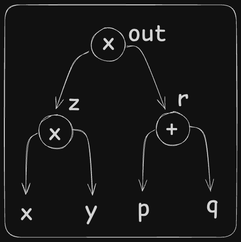
When the circuit is executed, all these variables take concrete values, forming the execution trace with which the proof is generated. This is the trace when $x = 2$, $y = 3$, $p = 4$ and $q = 5$:
| A | B | C |
|---|---|---|
| 2 | 3 | 6 |
| 4 | 5 | 9 |
| 6 | 9 | 54 |
Using this trace, we can now introduce the gate constraint, encoding the gate operation and ensuring correct execution. This is the vanilla PLONK gate equation:
$$q_L a + q_R b + q_O c + q_M (a b) + q_C = 0$$
where $a, b$ and $c$ are the left, right and output wires of the gate.
- To say $a + b = c$, we let $q_L$ and $q_R$ equal $1$, and $q_O$ equal $-1$. The other coefficients aren't used, so we set $q_M$ and $q_C$ to $0$.
- To say $a \times b = c$, we set $q_O$ to $-1$, $q_M$ to $1$, and the rest of the coefficients to $0$.
- To bind a wire to a public constant $k$, we let $q_L$ equal $1$, $q_C$ equal $-k$, and the rest equal $0$, so that the gate reads $a - k = 0$.
For the 3 gates we are working with, the gate equations look like this, and each one holds:
- Gate 1: $0 \cdot 2 + 0 \cdot 3 - 1 \cdot 6 + 1 \cdot (2 \cdot 3) + 0 = 0$
- Gate 2: $1 \cdot 4 + 1 \cdot 5 - 1 \cdot 9 + 0 \cdot (4 \cdot 5) + 0 = 0$
- Gate 3: $0 \cdot 6 + 0 \cdot 9 - 1 \cdot 54 + 1 \cdot (6 \cdot 9) + 0 = 0$
Next, we collect all these values into vectors, so we can build one relationship with which the protocol can progress:
$$q_L = (0, 1, 0) \quad q_R = (0, 1, 0) \quad q_O = (-1, -1, -1)$$
$$q_M = (1, 0, 1) \quad q_C = (0, 0, 0)$$
$$a = (2, 4, 6) \quad b = (3, 5, 9) \quad c = (6, 9, 54)$$
Next we interpolate these vectors to obtain polynomials, over the domain of roots of unity. But our example has a small problem: the vectors have size $3$, which is not a power of $2$, and we need a power of two to get a suitable multiplicative subgroup. To solve this, we extend the vectors with zeros, which is an empty gate that trivially holds, and interpolate over the roots of unity with $n = 4$:
$$q_L = (0, 1, 0, 0) \quad q_R = (0, 1, 0, 0) \quad q_O = (-1, -1, -1, 0)$$
$$q_M = (1, 0, 1, 0) \quad q_C = (0, 0, 0, 0)$$
$$a = (2, 4, 6, 0) \quad b = (3, 5, 9, 0) \quad c = (6, 9, 54, 0)$$
Using this technique, we can capture the whole execution trace with these 8 polynomials, no matter how big the circuit is.
But there is one more thing! We have only shown that each gate is satisfied, not how the gates are wired to each other. This introduces us to "copy constraints".
Copy Constraints
Copy constraints ensure that certain wire values are equal across different parts of a circuit, without revealing the actual values. For example, the output of gate 1 must be the same value as the left input of gate 3.
We check that the wire values are copied correctly using a permutation argument (Bayer and Groth, 2012).
The permutation check
Label the positions $1, \ldots, 5$, with wire values $w = (5, 10, 2, 5, 5)$, where positions 1, 4 and 5 must hold the same value. Pick a permutation that cycles through the positions that must match: $\sigma = (5, 2, 3, 1, 4)$. So position 1 maps to 5, position 4 maps to 1, and position 5 maps to 4.
Using random $\beta, \gamma$, combine each wire value with its position, and separately with its permuted position:
$$z_{1,i} = w_i + \beta i + \gamma \qquad z_{2,i} = w_i + \beta \sigma_i + \gamma$$
For our values:
$$z_1 = [5 + \beta + \gamma,\ 10 + 2\beta + \gamma,\ 2 + 3\beta + \gamma,\ 5 + 4\beta + \gamma,\ 5 + 5\beta + \gamma]$$
$$z_2 = [5 + 5\beta + \gamma,\ 10 + 2\beta + \gamma,\ 2 + 3\beta + \gamma,\ 5 + \beta + \gamma,\ 5 + 4\beta + \gamma]$$
These are the same list in a different order, so the check $\prod_i z_{1,i} / z_{2,i} = 1$ passes. If position 4 held 6 instead of 5, then $z_1$ would contain $6 + 4\beta + \gamma$ and $z_2$ would contain $6 + \beta + \gamma$. The lists would no longer match, and the check would fail, except with negligible probability over $\beta$ and $\gamma$.
Now that we have a good understanding of the permutation check, let's connect it to PLONK.
The best explanation of this concept I found was documented by the LambdaClass team, so I use the same approach to explain this wire relationship. We represent the circuit structure and the witness in the form of matrices.
Introducing the $Q$ matrix:
| $Q_L$ | $Q_R$ | $Q_M$ | $Q_O$ | $Q_C$ |
|---|---|---|---|---|
| 0 | 0 | 1 | -1 | 0 |
| 1 | 1 | 0 | -1 | 0 |
| 0 | 0 | 1 | -1 | 0 |
| 0 | 0 | 0 | 0 | 0 |
The $V$ matrix. The gate equations alone are not enough. This trace satisfies all of them, but it doesn't correspond to a valid execution, because the left input of the third gate is 7 rather than the 6 computed by the first gate:
| A | B | C |
|---|---|---|
| 2 | 3 | 6 |
| 4 | 5 | 9 |
| 7 | 9 | 63 |
The $V$ matrix encodes how the result of one gate is carried to an input of a later one. These are called wirings. Like the $Q$ matrix, it's independent of any individual evaluation. It holds an index for each input and intermediate variable. In this case (leaving out the empty padding row):
| L | R | O |
|---|---|---|
| 1 | 2 | 0 |
| 4 | 5 | 3 |
| 0 | 3 | 6 |
Here $0$ is the index of $z$, $1$ of $x$, $2$ of $y$, $3$ of $r$, $4$ of $p$, $5$ of $q$, and $6$ of $out$. Now we can state a claim that is "if and only if".
New PLONK claim: Let $T$ be a matrix with columns $A, B, C$. It corresponds to a proper evaluation of the circuit if and only if:
- For all $i$, the following equality holds: $Q_{Li} A_i + Q_{Ri} B_i + Q_{Oi} C_i + Q_{Mi} (A_i B_i) + Q_{Ci} = 0$
- For all $i, j, k, l$ such that $V_{i,j} = V_{k,l}$, we have $T_{i,j} = T_{k,l}$. This is the copy constraint.
With this, we can encode the circuit execution and enforce its wiring, which is just what we need.
In zero-knowledge proof protocols, we almost always operate on polynomials, so we need to convert these claims into polynomial equations.
Starting with claim 1
Let $\omega$ be a primitive $N$-th root of unity, and let $H = \{\omega^i : 0 \leq i < N\}$. Let $a, b, c, q_L, q_R, q_M, q_O, q_C$ be the polynomials of degree less than $N$ that interpolate the columns $A, B, C, Q_L, Q_R, Q_M, Q_O, Q_C$ on the domain $H$. This means, for example, that $a(\omega^i) = A_i$ for all $i$, and similarly for the other columns.
With this, claim 1 can be expressed as:
$$a(x) q_L(x) + b(x) q_R(x) + a(x) b(x) q_M(x) + c(x) q_O(x) + q_C(x) = 0 \quad \text{for all } x \in H$$
Interestingly, in the world of polynomials, this is equivalent to the left side being divisible by the polynomial that vanishes on $H$. So there is a polynomial $t$ with:
$$a q_L + b q_R + a b q_M + c q_O + q_C = Z_H\, t, \quad \text{where } Z_H(X) = X^N - 1$$
Transforming claim 2
Recall the permutation check. A permutation is a rearrangement of a set, usually denoted $\sigma$. In our case, the set is all position pairs:
$$I = \{(i, j) : 0 \leq i < N,\ 0 \leq j < 3\}$$
where $i$ is the row and $j$ is the column. The matrix $V$ induces a permutation of this set: $\sigma((i, j))$ is the position of the next occurrence of the value at $(i, j)$, and after the last occurrence it goes back to the first. Recall $V$ is:
| L | R | O |
|---|---|---|
| 1 | 2 | 0 |
| 4 | 5 | 3 |
| 0 | 3 | 6 |
The permutation for this case is:
- $\sigma((0,0)) = (0,0)$
- $\sigma((0,1)) = (0,1)$
- $\sigma((0,2)) = (2,0)$
- $\sigma((1,0)) = (1,0)$
- $\sigma((1,1)) = (1,1)$
- $\sigma((1,2)) = (2,1)$
- $\sigma((2,0)) = (0,2)$
- $\sigma((2,1)) = (1,2)$
- $\sigma((2,2)) = (2,2)$
Claim 2 can now be expressed as: for all $(i,j) \in I$, $T_{i,j} = T_{\sigma((i,j))}$. This means that the sets $A$ and $B$ below are equal:
$$A = \{((i,j), T_{i,j}) : (i,j) \in I\}$$
$$B = \{(\sigma((i,j)), T_{i,j}) : (i,j) \in I\}$$
This is great, but we would like to represent claim 2 as a polynomial identity, which is more convenient for the protocol. The solution introduces the concept of equality of sets.
First, explore this, a deep dive into multiset equality checks, for a very good overview before we continue.
Equality of Sets
Problem: how do we check if two multisets $A = \{a_0, a_1, \ldots, a_{k-1}\}$ and $B = \{b_0, b_1, \ldots, b_{k-1}\}$ of field elements are equal?
Naive attempt: multiplication
You might think to multiply all the elements of $A$ and $B$, and compare the results:
$$\prod_{i=0}^{k-1} a_i \quad \text{and} \quad \prod_{i=0}^{k-1} b_i$$
This test fails in some cases. For instance, $A = \{4, 15\}$ and $B = \{6, 10\}$ both give a product of $60$, but clearly $A \neq B$.
Better approach: polynomials
Instead of comparing products, we use polynomials whose roots represent the sets. For $A$, construct:
$$f_A(X) = (a_0 + X)(a_1 + X) \cdots (a_{k-1} + X)$$
and do the same for $B$:
$$f_B(X) = (b_0 + X)(b_1 + X) \cdots (b_{k-1} + X)$$
The multisets $A$ and $B$ are equal if and only if $f_A(X) = f_B(X)$, which holds because of unique factorization of polynomials.
Checking equality efficiently
Instead of comparing the polynomials symbolically, we use a random evaluation. Pick a random field element $\gamma$ and evaluate $f_A(\gamma)$ and $f_B(\gamma)$. If they are equal then, with high probability, $A = B$.
This relies on the Schwartz-Zippel lemma, which says that two distinct polynomials are equal at a random point only with very small probability.
Encoding the product with roots of unity
A verifier can't multiply all those terms itself, so we use a special domain $H$ based on the roots of unity. Define:
- $\omega$: A primitive $k$-th root of unity.
- $H = \{1, \omega, \omega^2, \ldots, \omega^{k-1}\}$: The evaluation points.
For $A$, construct the polynomial $f$ that interpolates the values $\{a_0 + \gamma, a_1 + \gamma, \ldots, a_{k-1} + \gamma\}$ on $H$. Similarly, construct $g$ for $B$.
Now introduce a polynomial $Z(X)$, a running product of the ratios, with:
$$Z(1) = 1 \qquad \text{and} \qquad Z(h) f(h) = g(h) Z(\omega h) \quad \forall h \in H$$
Walking around the domain and returning to the start, these conditions can only hold if:
$$\prod_{i=0}^{k-1} (a_i + \gamma) = \prod_{i=0}^{k-1} (b_i + \gamma)$$
Note: if you find $g(X)Z(\omega X)$ confusing, explore this.
The next thing to do is extend this from a set of field elements to a set of tuples of field elements, which gets us much closer to the Plonkish permutation argument.
Lemma
Let $A = \{\bar{a}_0, \ldots, \bar{a}_{k-1}\}$ and $B = \{\bar{b}_0, \ldots, \bar{b}_{k-1}\}$ be multisets of pairs of field elements, where $\bar{a}_i = (a_{i,0}, a_{i,1})$ and similarly for $\bar{b}_i$.
- Mapping tuples to field elements: Let $\beta, \gamma \in \mathbb{F}$ be random field elements. Each pair is mapped to a single field element, $a_{i,0} + a_{i,1}\beta + \gamma$, and similarly for $B$.
- Interpolating polynomials: With $H$ as above, construct $f(X)$ and $g(X)$ that interpolate those mapped values for $A$ and $B$ respectively on $H$.
- Equality verification: Check for the existence of a polynomial $Z(X)$ satisfying $Z(\omega^0) = 1$, and $Z(h) f(h) = g(h) Z(\omega h)$ for all $h \in H$.
If such a polynomial $Z(X)$ exists then, with overwhelming probability over $\beta$ and $\gamma$, the multisets $A$ and $B$ are equal.
Applying This to PLONK
Recall the sets from claim 2:
$$A = \{((i,j), T_{i,j}) : (i,j) \in I\} \qquad B = \{(\sigma((i,j)), T_{i,j}) : (i,j) \in I\}$$
Their elements include an index pair $(i, j)$, not a field element, so we can't apply the lemma yet. We need to convert them.
Mapping indexed pairs to field elements
For each element $((i, j), v)$, we leave $v$ as it is, and map the index $(i, j)$ to a field element such that different index pairs map to distinct field elements. Let $\eta$ be a primitive $3N$-th root of unity, and map $((i, j), v)$ to the pair $(\eta^{3i + j}, v)$.
Using this mapping, the sets become:
$$A = \{(\eta^{3i + j}, T_{i,j}) : (i,j) \in I\}$$
$$B = \{(\eta^{3k + l}, T_{i,j}) : (i,j) \in I,\ \sigma((i,j)) = (k,l)\}$$
Claim 2 is equivalent to the equality of these two sets.
Equality verification via polynomials
Let $\beta, \gamma \in \mathbb{F}$ be random, and $D = \{1, \eta, \eta^2, \ldots, \eta^{3N-1}\}$. Define $f(X)$ and $g(X)$ as the polynomials interpolating these values on $D$:
$$f \text{ interpolates } \{T_{i,j} + \eta^{3i + j}\beta + \gamma : (i,j) \in I\}$$
$$g \text{ interpolates } \{T_{i,j} + \eta^{3k + l}\beta + \gamma : (i,j) \in I,\ \sigma((i,j)) = (k,l)\}$$
If there exists a polynomial $Z(X)$ such that
$$Z(\eta^0) = 1 \qquad \text{and} \qquad Z(d) f(d) = g(d) Z(\eta d) \quad \forall d \in D$$
then the sets $A$ and $B$ are equal with overwhelming probability.
Moving to the smaller domain
Let $\omega = \eta^3$, a primitive $N$-th root of unity, and $H = \{1, \omega, \ldots, \omega^{N-1}\}$. Since $\eta^{3i+j} = \omega^i \eta^j$, the three columns of row $i$ have the indices $\omega^i$, $\eta\, \omega^i$ and $\eta^2 \omega^i$. Three distinct shifts of $H$ like these are written $H$, $k_1 H$ and $k_2 H$, so here $k_1 = \eta$ and $k_2 = \eta^2$. The protocol can then take three steps of the running product at once, one row at a time, and work over $H$ alone. That gives the $z$ polynomial of the prover's second round.
Define $S_{\sigma_1}, S_{\sigma_2}, S_{\sigma_3}$ as the interpolations on $H$ of these values:
$$S_{\sigma_1} : \{\eta^{3k + l} : (i, 0) \in I,\ \sigma((i, 0)) = (k, l)\}$$
$$S_{\sigma_2} : \{\eta^{3k + l} : (i, 1) \in I,\ \sigma((i, 1)) = (k, l)\}$$
$$S_{\sigma_3} : \{\eta^{3k + l} : (i, 2) \in I,\ \sigma((i, 2)) = (k, l)\}$$
Before concluding, we clearly define the structure CommonPreprocessedInput, which holds everything fixed by the circuit, and is essential in the proof generation phase:
CommonPreprocessedInput $\{ S_{\sigma_1}, S_{\sigma_2}, S_{\sigma_3}, q_L, q_R, q_O, q_M, q_C \}$
The witness polynomials $a, b, c$ are not part of it, since they change with every execution.
With these, PLONKish arithmetization is complete.
References (these resources are life savers):