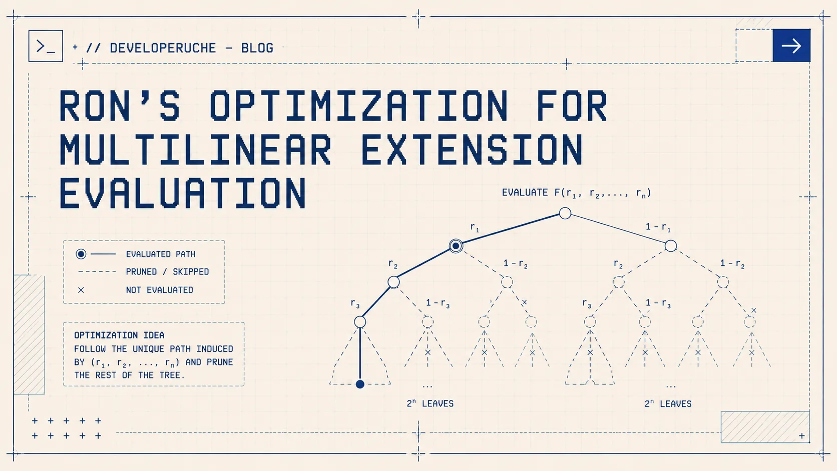
Author's Note: This article builds directly on concepts established in Part 1: Multilinear Polynomial Extension and Direct Evaluation. If you haven't read that yet, I strongly advise starting there to understand the definition of the MLE and the naive direct evaluation method. This part focuses on optimization strategies proposed by Ron Rothblum.
In Part 1, we implemented the "Direct Evaluation" of a Multilinear Extension (MLE). While mathematically clear, that approach suffers from a significant bottleneck: it requires $O(m \cdot 2^m)$ field multiplications.
In the context of Zero-Knowledge Proofs (like Spartan or checking Sumcheck protocols), the prover often works with large polynomials ($m \approx 20+$). At this scale, the difference between $m \cdot 2^m$ and $2^m$ is a factor of 20x or more. Standard Dynamic Programming (DP) can achieve $O(2^m)$ speed but often at the cost of $O(2^m)$ memory—a prohibitive cost for large zkVMs.
In this post, we explore an elegant optimization I call Ron’s Method (from Rothblum). This technique allows us to evaluate the MLE in linear time $O(2^m)$ with constant extra memory $O(1)$ (relative to the input size) by utilizing Gray Codes.
The Intuition: Streaming the Hypercube
Recall the MLE formula:
$$ \tilde{f}(z) = \sum_{b \in \{0,1\}^m} \text{eq}(z, b) \cdot f(b) $$
The Lagrange basis term $\text{eq}(z, b)$ is a product of $m$ univariate terms. In the standard lexicographic iteration (000, 001, 010...), consecutive points $b$ and $b'$ might differ by multiple bits. For example, moving from 011 to 100 flips 3 bits. This forces us to recompute the product almost entirely.
However, if we iterate over the hypercube using a Gray Code sequence, consecutive integers differ by exactly one bit. This mathematical property allows us to update our running product $\text{eq}(z, b)$ with a single multiplication operation.
The Update Logic
Let $b$ and $b'$ be two adjacent points in a Gray code sequence that differ only at index $k$. To transition from $\text{eq}(z, b)$ to $\text{eq}(z, b')$, we don't need to rebuild the product. We simply "swap out" the term for the $k$-th coordinate.
We precompute two update ratios for every dimension $i \in \{0, \dots, m-1\}$:
$$ eq(z, b \oplus e_i) = eq(z, b) \cdot \frac{eq_1(z_i, b_i \oplus 1)}{eq_1(z_i, b_i)} $$
By precomputing these ratios, we can transition from one basis evaluation to the next with one multiplication.
- Flip $0 \to 1$ (Up): $R_{i, \uparrow} = \frac{z_i}{1 - z_i}$
- Flip $1 \to 0$ (Down): $R_{i, \downarrow} = \frac{1 - z_i}{z_i}$
(Note: We assume $z_i \notin \{0,1\}$ for now. We will handle the boolean case in the "Dimension Reduction" section).
The update rule becomes:
$$ \text{eq}(z, b') = \text{eq}(z, b) \times (\text{Ratio for bit } k) $$
Visualizing the Traversal
Let's trace this with a concrete example where $m=3$. We want to compute the weighted sum of evaluations $f(b)$.
- Dimensions ($m$): 3
- Verifier Challenge ($z$): $z = (z_0, z_1, z_2)$ (using 0-indexing for convenience).
- Evaluations ($f$): A vector $[0, 1, 2, 3, 4, 5, 6, 7]$.
- Note: These values typically map to lexicographic indices $000_2$ to $111_2$. Because we are traversing in Gray code order, we must access these values out of order.
1. Precomputation We calculate the update ratios for each dimension $i \in \{0, 1, 2\}$. Assuming $z_i \notin \{0, 1\}$:
- To flip bit $i$ from $0 \to 1$: multiply by $R_{i, \uparrow} = \frac{z_i}{1-z_i}$
- To flip bit $i$ from $1 \to 0$: multiply by $R_{i, \downarrow} = \frac{1-z_i}{z_i}$
2. The Traversal
- Start at $b=000$.
- Initial accumulator $E = (1-z_0)(1-z_1)(1-z_2)$.
- We traverse the Gray code sequence.
| Step | Gray Code ($b$) | Bit Flipped | Action on $E$ | Contribution to Sum |
|---|---|---|---|---|
| 0 | 000 | — | Initial Calc | $E \cdot f(0)$ |
| 1 | 001 | 0 ($0 \to 1$) | $E \times R_{0, \uparrow}$ | $E \cdot f(1)$ |
| 2 | 011 | 1 ($0 \to 1$) | $E \times R_{1, \uparrow}$ | $E \cdot f(3)$ |
| 3 | 010 | 0 ($1 \to 0$) | $E \times R_{0, \downarrow}$ | $E \cdot f(2)$ |
| 4 | 110 | 2 ($0 \to 1$) | $E \times R_{2, \uparrow}$ | $E \cdot f(6)$ |
| 5 | 111 | 0 ($0 \to 1$) | $E \times R_{0, \uparrow}$ | $E \cdot f(7)$ |
| 6 | 101 | 1 ($1 \to 0$) | $E \times R_{1, \downarrow}$ | $E \cdot f(5)$ |
| 7 | 100 | 0 ($1 \to 0$) | $E \times R_{0, \downarrow}$ | $E \cdot f(4)$ |
Notice that for every step after the initialization, we perform exactly one field multiplication to update our weight $E$, and one addition to accumulate the result. This is optimal.
3. Detailed Trace of the Math We track the accumulator $E$ as it transforms through the hypercube.
- Definitions:
- $R_{i, \uparrow} = \frac{z_i}{1-z_i}$ (multiplier when bit $i$ flips $0 \to 1$).
- $R_{i, \downarrow} = \frac{1-z_i}{z_i}$ (multiplier when bit $i$ flips $1 \to 0$).
- Target index $b$ is written as $(b_2, b_1, b_0)_2$.
Step 0: Initialization
- Gray Code:
000(Integer 0) - Action: Compute the base term directly.
- Math:
$$E_0 = (1-z_2)(1-z_1)(1-z_0)$$
- Result: Matches $eq(z, 000)$.
- Accumulate: Add $E_0 \cdot f(0)$ to sum.
Step 1: Flip Bit 0 ($0 \to 1$)
- Gray Code:
001(Integer 1) - Action: Update $E_0$ using ratio $R_{0, \uparrow}$.
- Math:
$$E_1 = E_0 \cdot \frac{z_0}{1-z_0}$$
$$E_1 = (1-z_2)(1-z_1)\cancel{(1-z_0)} \cdot \frac{z_0}{\cancel{1-z_0}}$$
- Result: $(1-z_2)(1-z_1)z_0$. Matches $eq(z, 001)$.
- Accumulate: Add $E_1 \cdot f(1)$ to sum.
Step 2: Flip Bit 1 ($0 \to 1$)
- Gray Code:
011(Integer 3) - Action: Update $E_1$ using ratio $R_{1, \uparrow}$.
- Math:
$$E_2 = E_1 \cdot \frac{z_1}{1-z_1}$$
$$E_2 = (1-z_2)\cancel{(1-z_1)}z_0 \cdot \frac{z_1}{\cancel{1-z_1}}$$
- Result: $(1-z_2)z_1 z_0$. Matches $eq(z, 011)$.
- Accumulate: Add $E_2 \cdot f(3)$ to sum. Note: We access index 3 here, not 2.
Step 3: Flip Bit 0 ($1 \to 0$)
- Gray Code:
010(Integer 2) - Action: Update $E_2$ using ratio $R_{0, \downarrow}$.
- Math:
$$E_3 = E_2 \cdot \frac{1-z_0}{z_0}$$
$$E_3 = (1-z_2)z_1 \cancel{z_0} \cdot \frac{1-z_0}{\cancel{z_0}}$$
- Result: $(1-z_2)z_1 (1-z_0)$. Matches $eq(z, 010)$.
- Accumulate: Add $E_3 \cdot f(2)$ to sum.
Step 4: Flip Bit 2 ($0 \to 1$)
- Gray Code:
110(Integer 6) - Action: Update $E_3$ using ratio $R_{2, \uparrow}$.
- Math:
$$E_4 = E_3 \cdot \frac{z_2}{1-z_2}$$
$$E_4 = \cancel{(1-z_2)}z_1 (1-z_0) \cdot \frac{z_2}{\cancel{1-z_2}}$$
- Result: $z_2 z_1 (1-z_0)$. Matches $eq(z, 110)$.
- Accumulate: Add $E_4 \cdot f(6)$ to sum.
Step 5: Flip Bit 0 ($0 \to 1$)
- Gray Code:
111(Integer 7) - Action: Update $E_4$ using ratio $R_{0, \uparrow}$.
- Math:
$$E_5 = E_4 \cdot \frac{z_0}{1-z_0}$$
$$E_5 = z_2 z_1 \cancel{(1-z_0)} \cdot \frac{z_0}{\cancel{1-z_0}}$$
- Result: $z_2 z_1 z_0$. Matches $eq(z, 111)$.
- Accumulate: Add $E_5 \cdot f(7)$ to sum.
Step 6: Flip Bit 1 ($1 \to 0$)
- Gray Code:
101(Integer 5) - Action: Update $E_5$ using ratio $R_{1, \downarrow}$.
- Math:
$$E_6 = E_5 \cdot \frac{1-z_1}{z_1}$$
$$E_6 = z_2 \cancel{z_1} z_0 \cdot \frac{1-z_1}{\cancel{z_1}}$$
- Result: $z_2 (1-z_1) z_0$. Matches $eq(z, 101)$.
- Accumulate: Add $E_6 \cdot f(5)$ to sum.
Step 7: Flip Bit 0 ($1 \to 0$)
- Gray Code:
100(Integer 4) - Action: Update $E_6$ using ratio $R_{0, \downarrow}$.
- Math:
$$E_7 = E_6 \cdot \frac{1-z_0}{z_0}$$
$$E_7 = z_2 (1-z_1) \cancel{z_0} \cdot \frac{1-z_0}{\cancel{z_0}}$$
- Result: $z_2 (1-z_1) (1-z_0)$. Matches $eq(z, 100)$.
- Accumulate: Add $E_7 \cdot f(4)$ to sum.
At the end of this linear scan, we have computed $\hat{f}(z)$ using exactly 7 multiplications for the updates (plus initial setup) and 8 additions for the accumulation.
The algorithm described so far assumes that $z_i \notin \{0, 1\}$ to avoid division by zero during the update steps. However, in real-world protocols (like Sumcheck), it is common for the verifier's challenge vector $z$ to contain boolean values (0 or 1), or for the engineer to want to evaluate the extension on a sub-cube.
The paper provides a powerful optimization for this case: Dimension Reduction.
Dimension Reduction
If a coordinate $z_i$ is boolean ($0$ or $1$), the Lagrange basis polynomial $eq_1(z_i, b_i)$ collapses:
- If $z_i = 1$, then $eq_1(1, b_i)$ is $1$ only if $b_i = 1$, and $0$ otherwise.
- If $z_i = 0$, then $eq_1(0, b_i)$ is $1$ only if $b_i = 0$, and $0$ otherwise.
Mathematically, we partition the coordinates into two sets:
- $S$ (Boolean Set): Indices where $z_i \in \{0, 1\}$.
- $\bar{S}$ (Non-Boolean Set): Indices where $z_i \in \mathbb{F} \setminus \{0, 1\}$.
The paper observes that $eq(z, b) = 0$ whenever the bits in $b$ do not exactly match the boolean values in $z$. Therefore, we can skip all vectors $b$ where $b_S \neq z_S$. We only perform the Gray code enumeration over the remaining coordinates in $\bar{S}$.
This effectively reduces the problem size from $2^m$ to $2^{|\bar{S}|}$, changing the complexity from exponential in $m$ to exponential only in the number of non-boolean variables.
Example when dimension reduction kicks in
Let's revisit our 3-variable example where $m=3$ and the full evaluation vector is indices $[0, \dots, 7]$.
Scenario: Suppose the verifier sends the challenge:
$$z = (z_0, z_1, z_2) = (0.5, 1, 0)$$
Here:
- $z_0 = 0.5$ (Non-boolean). This is the only "active" dimension we must iterate.
- $z_1 = 1$ (Boolean).
- $z_2 = 0$ (Boolean).
The Filtering Logic: We rely on the property that for the final result to be non-zero, the bits of our index $b = (b_2, b_1, b_0)_2$ must match the boolean constraints of $z$:
- Since $z_1 = 1$, we must have $b_1 = 1$.
- Since $z_2 = 0$, we must have $b_2 = 0$.
The only free variable is $b_0$.
The Reduced Iteration: Instead of iterating through all 8 indices ($000$ to $111$), we essentially fix $b_2=0$ and $b_1=1$, and iterate $b_0$ through its Gray code sequence ($0 \to 1$).
Our target indices are:
- $b = (0, 1, 0)_2 \to$ Index 2
- $b = (0, 1, 1)_2 \to$ Index 3
The Execution Trace: We are now computing a 1-variable MLE (over $z_0$) scaled by the fixed boolean terms (which evaluate to 1).
| Step | Active Bit ($b_0$) | Fixed Bits ($b_2, b_1$) | Full Index | Value Calculation |
|---|---|---|---|---|
| 0 | $0$ | $0, 1$ | 2 (010) | $Accum += f(2) \cdot (1-z_0)$ |
| 1 | $1$ | $0, 1$ | 3 (011) | $Accum += f(3) \cdot (z_0)$ |
We computed the exact result using only 2 steps instead of 8. In a large system (e.g., $m=20$), if half the variables are boolean, this optimization speeds up the prover by a factor of $2^{10} \approx 1000x$.
Ron Algo Impl Explaination
This is a high-performance implementation of Proposition 1 and Corollary 2 from Rothblum's note.
The code implements the core optimization: calculating the Multilinear Extension (MLE) in $O(2^m)$ time and $O(m)$ space using Gray code enumeration. It also implements the specific optimization for "general vectors" (where some $z_i \in \{0,1\}$) to reduce the problem size.
Here is the breakdown of the Rust code, linked directly to the theoretical steps in the paper.
1. The Precomputed Update Ratios
Code:
#[derive(Clone, Copy, Debug)]
pub struct UpdateRatio<F: Field> {
    up: F,   // Multiplier to flip 0 -> 1:  z / (1-z)
    down: F, // Multiplier to flip 1 -> 0:  (1-z) / z
}
Theory Connection: The paper states that consecutive terms in a Gray code sequence differ by exactly one bit. To update the running product $eq(z, b)$, we perform a single multiplication. The derivation comes from Equation (2) in the paper:
$$eq(z, b \oplus e_i) = \frac{eq_1(z_i, b_i \oplus 1)}{eq_1(z_i, b_i)} \cdot eq(z, b)$$
- If flipping $0 \to 1$: The multiplier is $\frac{z_i}{1-z_i}$ (variable
up). - If flipping $1 \to 0$: The multiplier is $\frac{1-z_i}{z_i}$ (variable
down).
The code precomputes these values to ensure the inner loop only performs one multiplication per step, fulfilling the requirement of exactly $2^m$ multiplications.
2\. Initialization and Handling Boolean Inputs
Code:
    let mut ratios = Vec::with_capacity(m);
    let mut active_bit_positions = Vec::with_capacity(m);
    let mut global_idx = 0usize;
    let mut current_eq = F::one();

    for (i, &val) in z.iter().enumerate() {
        let global_bit_pos = m - 1 - i; // Big-endian index adjustment

        if val.is_zero() {
            // Do nothing; bit remains 0 in global_idx
        } else if val.is_one() {
            global_idx |= 1 << global_bit_pos; // Fixed to 1
        } else {
            // General case: z_i is not 0 or 1
            let one_minus_val = F::one() - val;
            let r_up = val * one_minus_val.inverse().unwrap();
            let r_down = one_minus_val * val.inverse().unwrap();

            ratios.push(UpdateRatio { up: r_up, down: r_down });
            active_bit_positions.push(global_bit_pos);
            current_eq *= one_minus_val; // Initial value for b_i = 0
        }
    }
Theory Connection: This section implements the optimization for "general vectors" described in the proof of Proposition 1.
- Boolean Inputs ($z_i \in \{0,1\}$): The paper notes that $eq(z_S, b_S) = 0$ whenever $b_S \neq z_S$.
- The code efficiently skips these dimensions. It fixes the bits in
global_idx(effectively effectively "hard-coding" the correct path in the truth table) and does not add them toactive_bit_positions. This reduces the loop size from $2^m$ to $2^{|S|}$, where $|S|$ is the number of non-boolean variables.
- The code efficiently skips these dimensions. It fixes the bits in
- Initial
current_eq: The Gray code iteration starts at logical $00\dots0$. For the active variables, $eq_1(z_i, 0) = (1 - z_i)$. Therefore, the startingcurrent_eqis initialized to $\prod_{i \in Active} (1 - z_i)$.
3. The Gray Code Loop (The Core Algorithm)
Code:
    // ... setup code ...
    total_sum += current_eq * evals[global_idx]; // First term (all active bits 0)

    let mut prev_gray = 0usize;

    for k in 1..num_steps {
        // Standard Gray code generation: g(k) = (k >> 1) ^ k
        let gray = (k >> 1) ^ k;
        let diff = prev_gray ^ gray;

        // Identify which bit changed
        let active_idx = diff.trailing_zeros() as usize;
        let global_bit_pos = active_bit_positions[active_idx];

        // Determine direction of flip
        let direction_up = (gray & diff) != 0;

        if direction_up {
            current_eq *= ratios[active_idx].up;
        } else {
            current_eq *= ratios[active_idx].down;
        }

        // Update the truth table index
        global_idx ^= 1 << global_bit_pos;
        total_sum += current_eq * evals[global_idx];

        prev_gray = gray;
    }
Theory Connection: This loop implements the enumeration described in the proof: "We generate the sequence according to the Gray code ordering...".
let gray = (k >> 1) ^ k;: This generates the standard binary reflected Gray code.active_idx: This finds the index $i$ where the change occurred. Because we filtered out Boolean inputs, this index maps toactive_bit_positionsrather than the raw variable index.- The Update: The code executes the update rule: "store only the previous $eq(z,b)$ and update it using a single multiplication".
- If
direction_upis true, we flipped $0 \to 1$, so we multiply byup($z/(1-z)$). - Otherwise, we flipped $1 \to 0$, so we multiply by
down($(1-z)/z$).
- If
global_idx ^= 1 << global_bit_pos: This effectively "moves" our pointer in the truth tableevalsto the next required value without recalculating the index from scratch.
Summary on Impl Efficiency
- Multiplications: Exactly $2^{|Active|}$ multiplications inside the loop (one per iteration).
- Space: The
ratiosandactive_bit_positionsvectors consume $O(m)$ space, matching the paper's claim of linear space complexity. - Additions: Exactly $2^{|Active|}$ additions to
total_sum.
Performance Benchmarks
Theory suggests that Ron’s optimized method ($O(2^m)$) should strictly outperform the Direct method ($O(m \cdot 2^m)$). However, in systems programming, theory must always contend with CPU architecture, branch prediction, and memory hierarchy.
We implemented both methods in Rust using arkworks (BLS12-381 Fr field) and benchmarked them using criterion on an Apple Silicon machine.
The Results
| Variables ($m$) | Vector Size ($2^m$) | Direct Method | Ron's Optimized | Speedup Factor |
|---|---|---|---|---|
| 5 | 32 | 3.16 µs | 13.96 µs | 4x (Slower) |
| 10 | 1,024 | 170.43 µs | 54.62 µs | 3.12x |
| 17 | 131,072 | 37.42 ms | 4.68 ms | 7.99x |
| 20 | 1,048,576 | 341.27 ms | 102.17 ms | 3.34x |
The data reveals three distinct phases of performance behavior:
1. The Overhead Phase ($m=5$) At small sizes ($m=5$), the Optimized method is actually 4x slower than the naive approach.
- Why? The setup costs dominate. The Optimized method requires allocating vectors for ratios, computing inverses for $z_i$, and performing bitwise logic to generate Gray codes.
- The Lesson: For tiny sub-circuits or small lookups, the naive $O(m \cdot 2^m)$ approach is preferred because the constant factors are negligible and the code is instruction-cache friendly.
2. The Compute-Bound Phase ($m=10$ to $m=17$) This is the "sweet spot" where the algorithm shines.
- At $m=17$, we see an 8x speedup.
- Here, the vector size fits comfortably within the CPU's L2/L3 cache. The CPU is bound by arithmetic operations (field multiplications). By reducing the multiplications from $17 \cdot 2^{17}$ to $1 \cdot 2^{17}$, the theoretical efficiency translates directly to wall-clock time.
3. The Memory-Bound Phase ($m=20$) This tends to get less attension, At $m=20$, the speedup drops from ~8x to ~3.3x.
- The Context: A vector of $2^{20}$ BLS12-381 scalars (32 bytes each) occupies $\approx 33.5 \text{ MB}$. This exceeds the L3 cache size of most consumer CPUs.
- The Bottleneck: The "Direct" method iterates through the
evalsvector linearly (0, 1, 2...), which is perfect for the CPU's hardware prefetcher. - Ron's Method: While efficient in arithmetic, it traverses memory based on Gray codes (
000$\to$001$\to$011$\to$010). This results in a non-linear memory access pattern. Once the data size exceeds the cache, the CPU spends more cycles waiting for RAM (cache misses) than performing the field multiplications we optimized away.
My hot take
Ron’s optimization is a critical tool for modern zkVMs, particularly in the $m=10$ to $m=18$ range common in folding schemes and sumcheck protocols. However, engineers should remain aware of the "Memory Wall" at larger sizes ($m \ge 20$), where memory bandwidth may become the new bottleneck over arithmetic complexity.
References:
- *Rothblum, A Note on Efficient Computation of the Multilinear Extension
- Developeruche, Rust Impl